Feature matching

In this chapter, we will be matching AKAZE features and displaying the matches.

How do we perform feature matching?

Binary Features

As explained in the previous chapter, AKAZE's feature descriptors are comprised of bits. Each bit describes one comparison made between two points around the feature. These descriptors are generally designed so that similar features have similar descriptors. In this case, that means that similar features will have similar bit patterns. For AKAZE features, the number of bits that are different between two descriptors is the distance between them, and the number of bits in common is the similarity between them.

The primary reason that we use binary features is because computing the distance between two features is blazingly fast on modern computers. This allows us to get real-time performance. The amount of time that it takes to compare two binary features in practice is typically a few nanoseconds. Compare this to computing the distance between high dimensional (e.g., 128 dimensional for SIFT) floating point vectors, which typically takes much longer, even with modern SIMD instruction sets or the use of GPUs. How is this achieved?

How is the distance computed?

The way that the distance is computed can be summed up in two operations. The first operation is XOR. We simply take the XOR of the two 486-bit feature descriptors. The result has a 1 in every bit which is different between the two, and a 0 in every bit which is the same between the two. At this point, if you count the number of 1 in the output of the XOR, this actually tells us the distance between the two descriptors. This distance is called the hamming distance.

The next step we just need to count the number of 1 in the result, so how do we do that? Rust actually has a built-in method to do this on all primitive integers called count_ones.

How is this so fast?

We actually have an instruction on modern Intel CPUs called POPCNT. This will count the number of 1 in a 16-bit, 32-bit, or 64-bit number. This is actually incredibly fast, but it is possible to go faster.

To go faster, you can use SIMD instructions. Unfortunately, Intel has never introduced a SIMD POPCNT instruction, nor has ARM, thus we have to do this manually. Luckily, SIMD instructions have so many ways to accomplish things that we can hack our way to success. A paper was written on this topic called "Faster Population Counts Using AVX2 Instructions", but the original inspiration for this algorithm can be found here. The core idea of these algorithms is to use the PSHUFB instruction, added in SSSE3. This instruction lets us perform a vertical table look-up. In SIMD parlance, a vertical operation is one that performs the same operation on several segments of a SIMD register in parallel. The way the PSHUFB instruction from SSSE3 works is that it will let us perform a 16-way lookup. A 16-way lookup requires 4 input bits. The table we use is the population count operation for 4 bits. This means that 0b1000 maps to 1, 0b0010 maps to 1, 0b1110 maps to 3, and 0b1111 maps to 4. From there, we need to effectively perform a horizontal add to compute the output. In SIMD parlance, a horizontal operation is one which reduces (as in map-reduce) information within a SIMD register, and will typically reduce the dimensionality of the register. In this case, we want to add all of the 4-bit sums into one large sum. The method by which this is achieved is tedious, and the paper mentioned above complicates matters further by making it operate on 16 separate 256-bit vectors to increase speed further.

The lesson here is that SIMD can help us speed up various operations when we need to operate on lots of data in vectors. You should rely on libraries to take care of this or let the compiler optimize this out by using fixed size bit arrays where possible, although it wont be perfect. If you absolutely must squeeze that last bit of speed out because the problem demands it and you know your problem domain and preconditions well, then the rabbit hole goes deep, so feel free to explore the literature on population count. The XOR operation doesn't really get more complicated though, it's just an XOR, and everything supports XOR (that I know of).

Tricks often used when matching

Lowe's ratio test

Matching features has a few more tricks that are important to keep in mind. Notably, one of the most well-known tricks is the usage of the Lowe's ratio test, named after its creator David Lowe who offhandedly mentions it in the paper "Distinctive Image Features from Scale-Invariant Keypoints".

It is a recurring theme in computer vision that algorithms get named after the authors because they do not name algorithms which turn out to be incredibly important and fundamental. However, if we named every such algorithm that Richard Hartley created after himself, we would probably call this field Hartley Vision instead. Moving on...

The Lowe's ratio is very simple. When we compute the distance between a specific feature and several other features, some of those other features will have a smaller distance to this specific feature than others. In this case, we only care about the two best matching features, often called the two "nearest neighbors" or often abbreviated as 2-NN (k-NN in the general case). We simply want to see what the ratio is between the best distance and the second best distance. If this ratio is very small, that means that the feature you matched to is much better than the second best alternative, so it is more likely to be correct. Therefore, we just test to see if the ratio is below some threshold which is typically set to about 0.7.

The Lowe's ratio doesn't make as much sense for binary features. Consider that the distance between two independent features should be roughly 128-bits, and it should form a perfect binomial distribution. Additionally, the Lowe's ratio is typically applied to floating point vectors in euclidean space (L2 space), while binary features exist in hamming space. Therefore, with binary features, it may suffice to check that the best feature's distance is a certain number of bits better than the second best match. You can apply both the Lowe's ratio and this binary Lowe's test to more than just the first and best match specifically. It can also be applied to the best matches of the first and second best groups of matches to determine if one group may match a feature better than another group.

The Lowe's ratio test helps us filter outliers and only find discriminative matches.

Symmetric matching

Another important thing to do when matching is to match symmetrically. Typically, when you match features, you have two groups of features, the new ones and the ones you already have. With symmetric matching you are assuming that no feature appears twice in the new group and the group you already have. This can also be done in addition to the Lowe's ratio test. Conceptually, you can understand symmetric matching in the following way.

If you find the matches from the new group to the old group, that gives you a best match in the old group for each item in the new group.

If you find the matches from the old group to the new group, that gives you a best match in the new group for each item in the old group.

If the match in the new group and the match in the old group are only each other, then they are symmetric.

Another way to try and understand symmetric matching is with a visual aid. Consider a 1d line. Three features (X, Y, and Z) are in the following line: X-----Y-Z. Y is much closer to Z than to X. The closest match to X is Y, but the closest match to Y is Z. Therefore X and Y do not match symmetrically. However, Y and Z do form a symmetric match, because the closest point to Y is Z and the closest point to Z is Y. This analogy does not perfectly apply to our scenario as there aren't two separate groups, but the general concept still applies and can be used in other scenarios even outside of computer vision.

Symmetric matching helps filter outliers and only find discriminative matches, just like the Lowe's ratio test (or Lowe's distance test). When used together, they can be very powerful to filter outliers without even yet considering any geometric information.

Running the program

Make sure you are in the Rust CV mono-repo and run:

cargo run --release --bin chapter4-feature-matching

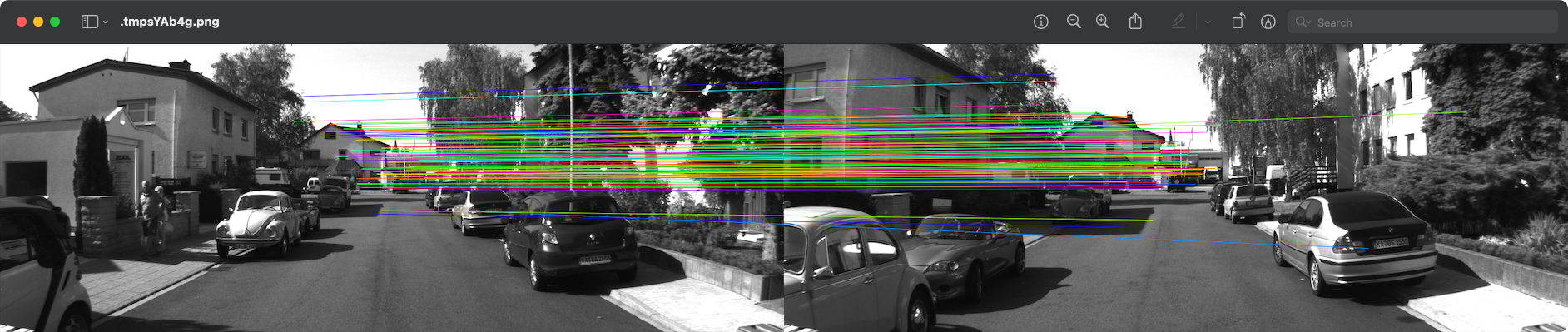
If all went well you should have a window and see this:

Matches

The code

Open two images of the same area


#![allow(unused)]
fn main() {
    let src_image_a = image::open("res/0000000000.png").expect("failed to open image file");
    let src_image_b = image::open("res/0000000014.png").expect("failed to open image file");
}

We already opened an image in the other chapters, but this time we are opening two images. Both images are from the same area in the Kitti dataset.

Extract features for both images and match them


#![allow(unused)]
fn main() {
    let akaze = Akaze::default();

    let (key_points_a, descriptors_a) = akaze.extract(&src_image_a);
    let (key_points_b, descriptors_b) = akaze.extract(&src_image_b);
    let matches = symmetric_matching(&descriptors_a, &descriptors_b);
}

We created an Akaze instance in the last chapter. We also extracted features as well, but this time two things are different. For one, this time we are keeping the descriptors and not just throwing them away. Secondly, we are extracting features from both images.

The next part is the most critical. This is where we match the features. We perform symmetric matching just as is explained above. The tutorial code has the full code for the symmetric matching procedure, and you can read through it if you are interested, but for now we will just assume it works as described. It also performs the "Lowe's distance test" mentioned above with the binary features. It is using a distance of 48 bits, which is quite large, but this results in highly accurate output data. Feel free to mess around with this number and see what kinds of results you get with different values.

Make a canvas


#![allow(unused)]
fn main() {
    let canvas_width = src_image_a.dimensions().0 + src_image_b.dimensions().0;
    let canvas_height = std::cmp::max(src_image_a.dimensions().1, src_image_b.dimensions().1);
    let rgba_image_a = src_image_a.to_rgba8();
    let rgba_image_b = src_image_b.to_rgba8();
    let mut canvas = RgbaImage::from_pixel(canvas_width, canvas_height, Rgba([0, 0, 0, 255]));
}

Here we are making a canvas. The first thing we do is we create a canvas with all black pixels. The canvas must be able to fit both images side-by-side, so that is taken into account when computing the width and height.

Render the images onto the canvas


#![allow(unused)]
fn main() {
    let mut render_image_onto_canvas_x_offset = |image: &RgbaImage, x_offset: u32| {
        let (width, height) = image.dimensions();
        for (x, y) in (0..width).cartesian_product(0..height) {
            canvas.put_pixel(x + x_offset, y, *image.get_pixel(x, y));
        }
    };
    render_image_onto_canvas_x_offset(&rgba_image_a, 0);
    render_image_onto_canvas_x_offset(&rgba_image_b, rgba_image_a.dimensions().0);
}

The first thing we do here is create a closure that will render an image onto the canvas at an X offset. This just goes through all X and Y combinations in the image using the cartesian_product adapter from the itertools crate. It puts the pixel from the image to the canvas, adding the X offset.

We then render image A and B onto the canvas. Image B is given an X offset of the width of image A. This is done so that both images are side-by-side.

Something that isn't shown here, but might be informative to some, is that because the last use of this closure is on this line, Rust will implicitly drop the lifetime constraint from the closure to the canvas, allowing us to mutate the canvas in the future. If we were to call this closure again on a later line then Rust might complain about borrowing rules. Rust does this to make coding in it more pleasant, but it can be confusing for beginners who may not have an intuition about how the borrow checker works.

Drawing lines for each match

This part is broken up to make it more manageable.


#![allow(unused)]
fn main() {
    for (ix, &[kpa, kpb]) in matches.iter().enumerate() {
        let ix = ix as f64;
        let hsv = Hsv::new(RgbHue::from_radians(ix * 0.1), 1.0, 1.0);
        let rgb = Srgb::from_color(hsv);
}

At this part we are iterating through each match. We also enumerate the matches so that we have an index. The index is converted to a floating point number. The reason we do this is so that we can assign a color to each index based on the index. This is done by rotating the hue of an HSV color by a fixed amount for each index. The HSV color has max saturation and value, so we basically get a bright and vivd color in all cases, and the color is modified using the radians of the hue. From this we produce an SRGB color, which is the color space typically used in image files unless noted otherwise.


#![allow(unused)]
fn main() {
        // Draw the line between the keypoints in the two images.
        let point_to_i32_tup =
            |point: (f32, f32), off: u32| (point.0 as i32 + off as i32, point.1 as i32);
        drawing::draw_antialiased_line_segment_mut(
            &mut canvas,
            point_to_i32_tup(key_points_a[kpa].point, 0),
            point_to_i32_tup(key_points_b[kpb].point, rgba_image_a.dimensions().0),
            Rgba([
                (rgb.red * 255.0) as u8,
                (rgb.green * 255.0) as u8,
                (rgb.blue * 255.0) as u8,
                255,
            ]),
            pixelops::interpolate,
        );
    }
}

This code is longer than its intention really is. First we create a closure that converts a keypoint's point, which is just a tuple of floats in sub-pixel position, into integers. It also adds a provided offset to the X value. This will be used to offset the points on image B when drawing match lines.

The next step is that we call the draw function. Note that for the first point we use the key point location from image A in the match and for the second point we use the key point location from image B in the match. Of course, we add an offset to image B since it is off to the right of image A. The rgb value is in floating point format, so we have to convert it to u8. This is done by multiplying by 255 and casting (which rounds down). The alpha value is set to 255 to make it totally solid. Unlike the previous chapters, this function doesn't support blending/canvas operation, so we just set the alpha to 255 to avoid it acting strange.

Display the resulting image

The rest of the code has been discussed in previous chapters. Go back and see them if you are curious how it works. All it does is save the matches image out and open it with your system's configured image viewer.

End

This is the end of this chapter.

Rust-CV Tutorials